The task of recognizing emotion in music, based on MFCCs features extracted from raw audio, was tackled from different perspectives and using Deep Neural Networks, aiming to gain insights into the field of Music Information Retrieval. Considering it a regression problem —predicting real values for valence and arousal— two approaches are studied: first, a single model is trained to predict both valence and arousal (further referred to as 2D-output) and second, a group of two models is trained, to separately predict valence and arousal, respectively (further referred to as 1D-output). Each approach is further extended to two experiments, the first involving training on the dataset as it is and the second involving augmentation of the original dataset prior to training. This project illustrates, through a comparative analysis of these experiments, the effects an imbalanced dataset has on the learning process, resulting in a collection of methods and observations, to be used further as starting point for a more comprehensive research.
The changes in amplitude over time (waveforms), representing music in its raw form, do not hold sufficient information for the emotion recognition task, such that feature extraction processes must be performed before feeding the data to a neural network.
In order to detect components of the audio signal, the features chosen for this study are the first 20 Mel Frequency Cepstral Coefficients (MFCCs). Being one of the most used representations in signal processing tasks, the MFCCs were first introduced in a 1980 study on monosyllabic word recognition [Davis & Mermelstein, 1980] . These are low-level features derived from the short-term Fourier Transform, that detect timbral and instrumentation aspects in an audio signal and are robust to variations in recording conditions.
The MFCCs features are extracted from the audio signal sampled at 44,100Hz/sec and divided in windows of 30ms duration without overlapping, using LibROSA, an open-source Python package for music and audio analysis.
Before using the resulting MFCCs features for training a neural network, a normalization operation must be performed. One of the most used techniques is Cepstral Mean and Variance Normalization, a simple computation of subtracting the mean and dividing this result by the standard deviation.
The dataset used in this project is The MediaEval Database for Emotional Analysis of Music [DEAM] , consisting in 1,744 song excerpts of ~45sec duration, with two types of annotations for valence and arousal available: dynamic —measured per second— and static —measured per 45sec. The static annotations, which are used in this study, are scaled down from range 1 .. 9 to range 0 .. 1. A visualization of data distribution in the 2D space of emotions shows an obvious imbalance in the four quadrants:
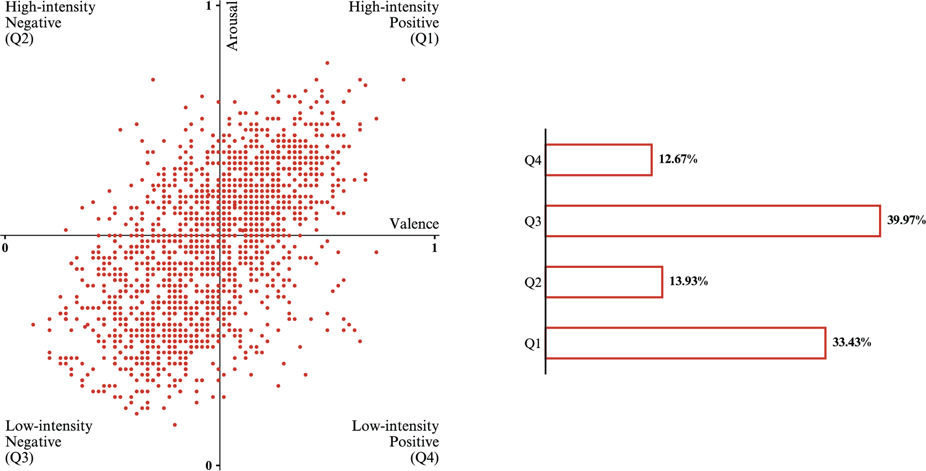
Distribution of DEAM data in the four quadrants.
The task of recognizing emotions in music is treated as a regression problem, the scope being to predict real values for valence and arousal dimensions of emotion. This strategy is further extended as follows:
There are also described two methods of working with the DEAM dataset, in the matter of data imbalance in quadrants:
The configurations used to tackle this task are build considering Convolutional Neural Networks architectures with 1D convolutions moving on the temporal dimension of the input and taking into account information across all channels, represented by the 20 MFCCs extracted from every windowed segment.
Few pre-processing steps on the audio data are required before extracting the MFCCs features: resampling the audio excerpts from DEAM dataset to the same sampling rate of 44100Hz and correcting the the differences in duration. To fix this difference, the samples longer than 45sec are cropped and in the case of the shorter samples, the last part of length equal to the difference to 45sec is copied to the right.
Using librosa library, the 20 MFCCs features are extracted from the waveforms, followed by normalization using Ceptral Mean and Variance normalization technique, resulting in data centered with zero mean and unit variance.
From the 1744 samples, the training is done on 80% of it and 20% is kept for testing the performance, resulting in the distribution in quadrants shown in the table below. The training and testing are done in batches of size 64, shuffled every epoch.

Original DEAM dataset - distribution in quadrants of the data in train and test sets.
The features extracted have the size 20×1500, where the first dimension represents the number of mel-coefficients and the second dimension represents the number of windowed segments obtained from the initial signal. To be fed to the 1D CNN, these 2D images representing MFCCs features will be considered 1D images with 20 channels.
For this approach, I considered a convolutional block with a 1D-Convolution layer with kernels of size 10 and stride 1, followed by Batch normalization, ReLU activation and subsampling by applying an Average Pooling layer with kernels of size 2 and stride 2.
The model has an architecture composed of two such convolutional blocks, followed by another subsampling process by adding an Average Pooling layer with kernel of size 10 and stride 10, thus reducing considerably the feature maps size, as a method of preventing the overfitting to occur. The flattened output of this layer is forwarded to a linear layer with 128 hidden units. Another regularization technique is represented by adding a Dropout layer with 50% probability. This is followed by ReLU activation and, finally, performing one more linear operation, the data is mapped to the 2D-output.
Given the properties of the averaging operation, the subsampling layer in the second convolutional block and subsampling layer succeeding the convolutional blocks are respresented as a single Avgerage Pooling layer with kernels of size and stride 20.
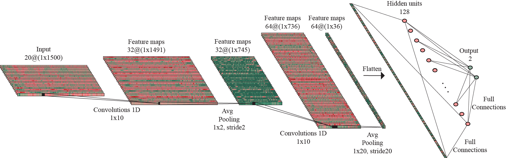
Architecture of the 2D-output model trained on the original dataset.
The optimization is performed using SGD for the cost computed with the MSE criterion, with scheduled decreases in learning rate. Observing the behavior of several configurations, the best strategy is learning less parameters for longer, mainly due to the fast occurrence of the overfitting phenomenon.
In order to understand the relation between the features chosen to represent the audio signal and emotion, R2 scores are computed for each of the two dimensions, displayed in the table below. It is visible that the MFCCs features have greater effect on the arousal dimension, when compared to the valence dimension.

Original DEAM dataset - R2 scores for 2D-output model.
Considering the different relations between the MFCCs features and the valence and arousal values, the next configuration consists in building two models to predict values in the two dimensions separately.
Starting with the same base scheme as previously mentioned, the two architectures differ in the number of parameters, as follows: the model that predicts valence uses 32 kernels for the first convolutional layer, 64 kernels for the second convolutional layer and 64 hidden units, while the model that predicts arousal has less parameters to be learned, with only 32 kernels for the second convolution. The only other difference in the 1D-output models architectures compared to the one of the 2D-output model is, as the names state, the mapping of the first linear layer to one output value instead of two.
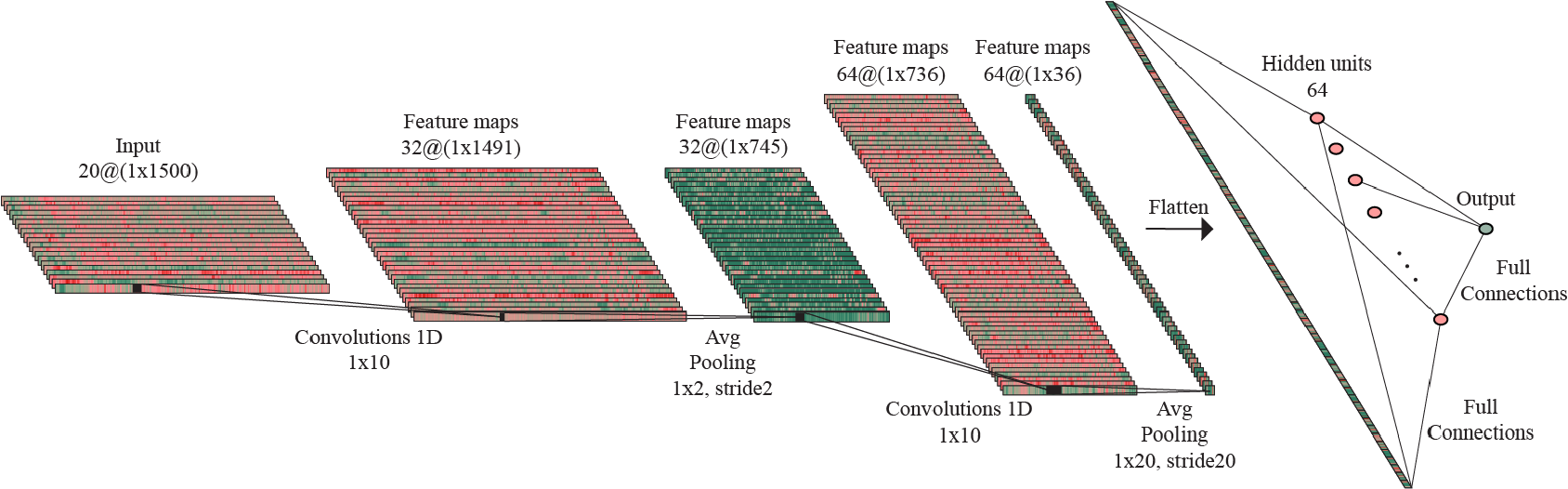
Architecture of the 1D-output model trained on the original dataset to predict valence.
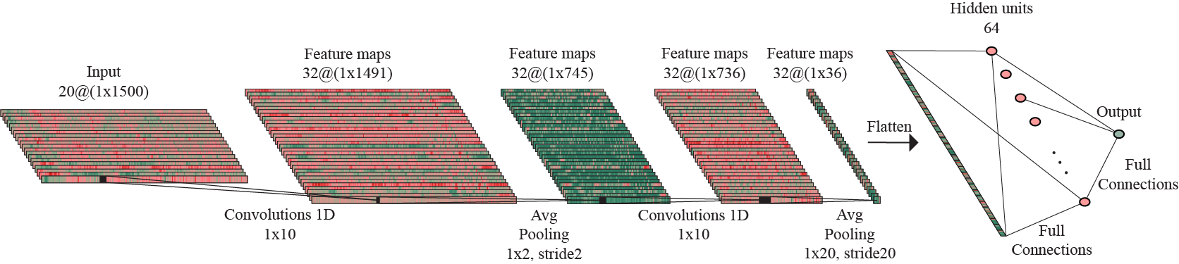
Architecture of the 1D-output model trained on the original dataset to predict arousal.
The results of the experiments based on the original DEAM dataset are further presented side-by-side, in a comparative manner, for better emphasis of the differences in performance. When referring to the configuration consisting in one model that predicts both valence and arousal values, the names 2D-output model and 2D-output CNN are used interchangeably, while 1D-output models and 1D-output CNNs are used when referring to the configuration consisting in two models that predict valence and arousal separately.
The first method for evaluating the models consists in computing the regression metrics MAE, MSE and R2 score for each dimension.

Original DEAM dataset - performance metrics for the 2D-output model and the 1D-output models.
The previously noted difference in the relations between the MFCCs features and the two emotion dimensions, given by the coefficient of correlation, remains valid in the case of the 1D-output configurations approach, with higher R2 score for the arousal predictions and lower R2 score for the valence predictions. Analysing the MAE and MSE errors values, there does not seem to be an improvement in the performance when training two models to predict separately on the two axes in the emotion space, compared to the first approach, of training a single model to predict values for both valence and arousal. It is possible, then, that the values in the two dimensions are not entirely independent.
For a better understanding of the results, the numeric scores are paired with visualizations of the predicted values compared to the observed values, with the results for each of the valence and arousal dimensions being presented in two types of plots.
In the cases of both the 2D-output model and the 1D-output models, it is visible that the values predicted cover a narrower range than the observed values.
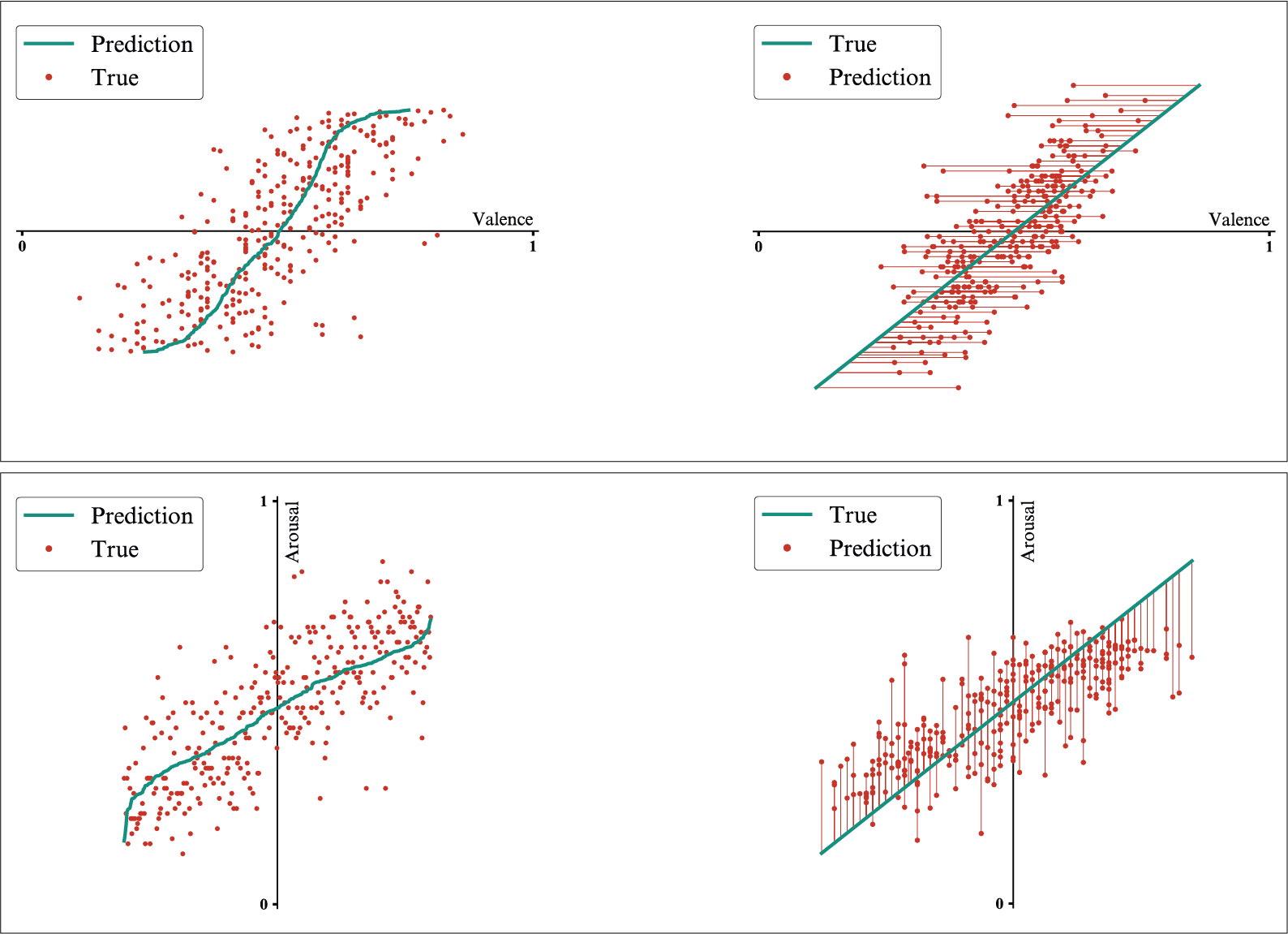
2D-output model trained on the original dataset - Results for the valence dimension (top) and for the arousal dimension (bottom).
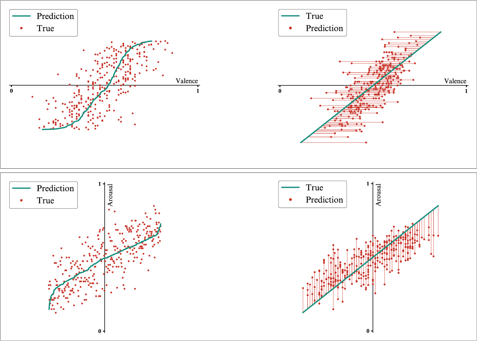
1D-output models trained on the original dataset - Results for the valence dimension (top) and for the arousal dimension (bottom).
This difference between the ranges of predicted and observed values is emphasized in the table below. In the case of the 2D-output model, very low and very high observed values of valence are predicted to be higher and lower, respectively, while for the arousal dimension, the observed values in the lower half of the range are predicted more accurately, but high values are predicted to be lower. This aspect is slightly improved when training two 1D models, especially in the case of valence prediction.

Original dataset - Ranges of the observed and predicted values for 2D-output and 1D-output models.
This may occur due to an imbalance in distribution of train data, this time in small intervals. For both dimensions —valence and arousal— the samples are spread similar to a Gaussian distribution, leaving the marginal intervals significantly underrepresented.
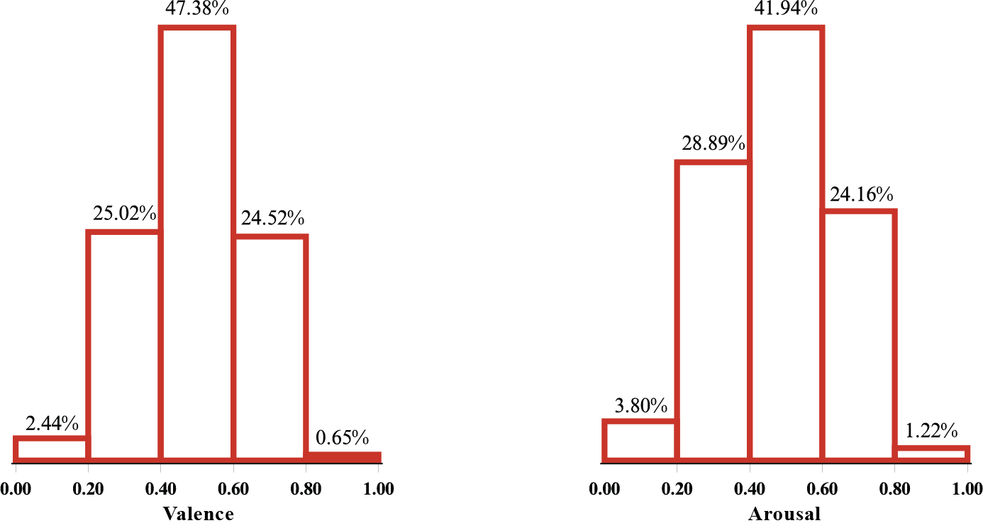
DEAM data distribution in intervals for valence and arousal dimensions.
Another observation comes as a consequence of the distribution of the data in DEAM dataset in the 2D space of emotions, regarding the faulty predictions for the observed values falling in quadrants 2 and 4.
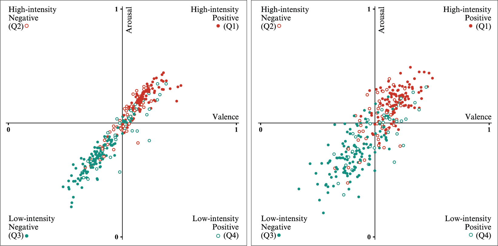
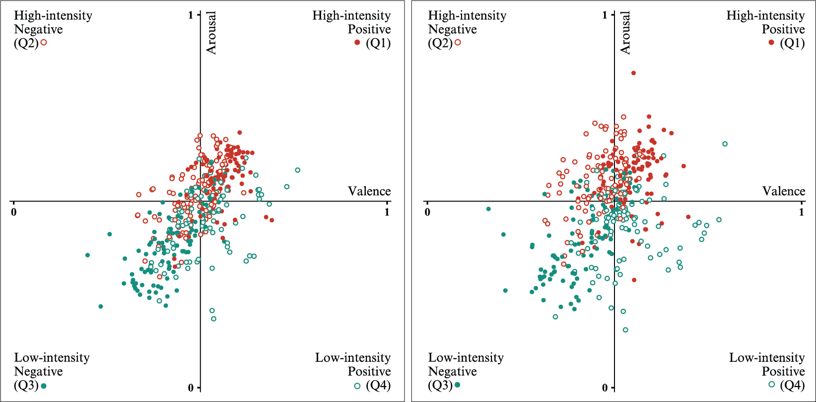
Original dataset - Result for valence and arousal in the space of emotions described by the four quadrants for the 2D-output model (left) and the 1D-output models (right).
Looking at the predictions localization in the figure above, it becomes clear that training a group of two models to output separately in the valence and arousal dimensions leads to an improvement in the spread of the predicted values in both the space of emotions in general and the underrepresented quadrants in particular. Therefore, although still far from ideal, the increase in the predictions accuracy for the observed values in quadrants 2 and 4 is worth mentioning. While, in the case of the 2D-output CNN approach, the accuracy is recorded to be 2.04% for quadrant 2 and 11.36% for quadrant 4, when predicting using the group of two 1D-output models it reaches 8.16% and 15.91%, respectively.
With the purpose of creating a balanced distribution of the data from DEAM dataset in the four quadrants describing the space of emotions, the previously preprocessed data is used. The first step in augmenting the dataset, is duplicating samples in underrepresented quadrants and removing samples in overrepresented ones, until a fixed size of 500 samples in each quadrant is reached. After this, the audio samples are reduced to 80% of their length, by choosing a start time for the cropped excerpt in a random fashion, resulting in samples of 36sec length.
Using the same parameters for the extraction of audio features as before, namely a window length of 30ms with no overlapping and 20 Mel-filters, the MFCCs obtained from each raw sample have the size 20×1200. These are treated as 1D images with 20 channels, being fed to CNNs with 1D convolutions.
Before training, the augmented dataset resulted is divided in train(1600 samples) and test(400 samples) sets, having an equal number of samples in each quadrant and the MFCCs features in each set are normalized considering the mean and variance computed on the train set. The training and testing are performed in batches of 64 samples, shuffled every epoch.
This method is based on the same configuration used when working with the original dataset, allowing for comparison between the two. Therefore, the architecture of the 2D-output model trained on the augmented dataset consists in two convolutional blocks, the difference lying in the dimensions of the feature maps. This sequence is followed by an Average Pooling layer, two linear operations, with a layer with 50% dropout probability of the data preceding the second one.

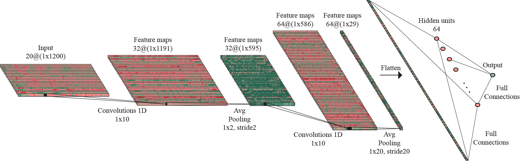
Architecture of the 2D-output model trained on the augmented dataset.
Approaching the task by training a group of two models on the augmented dataset, the same architectures designed for working with the original dataset are used. Keeping the same number of learnable parameters, the configurations differ in the dimensions of the feature maps, according to the smaller size of the input features. Hence, the model trained to predict valence has more parameters than the model trained to predict arousal.
Architecture of the 1D-output model trained on the augmented dataset to predict valence.
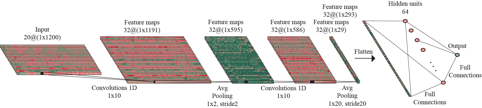
Architecture of the 1D-output model trained on the augmented dataset to predict arousal.
As before, the results for the experiments based on the augmented DEAM dataset are presented comparatively and the same naming conventions are used: 2D-output model and 2D-output CNN are used interchangeably when referring to the configuration consisting in one model that predicts both valence and arousal values, while 1D-output models and 1D-output CNNs are used when referring to the configuration consisting in two models that predict valence and arousal separately.
Computing the first set of performance metrics, the R2 highlight again the milder influence the MFCCs features have on the valence dimensions, when compared to their stronger influence on the arousal dimension. The MAE and MSE errors values show a significant improvement in the values predicted using the two 1D-output models, in contrast with the 2D-output model.

Augmented DEAM dataset - performance metrics for 2D-output model and the 1D-output models.
Analysing the visualizations of the observed and predicted values in the valence and arousal dimensions for the 2D-output model and the 1D-output models, the superiority of the latter is once again visible, considering the goodness of fit.
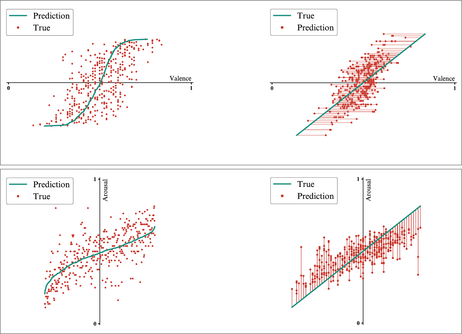
2D-output model trained on the augmented dataset - Results for the valence dimension (top) and for the arousal dimension (bottom).
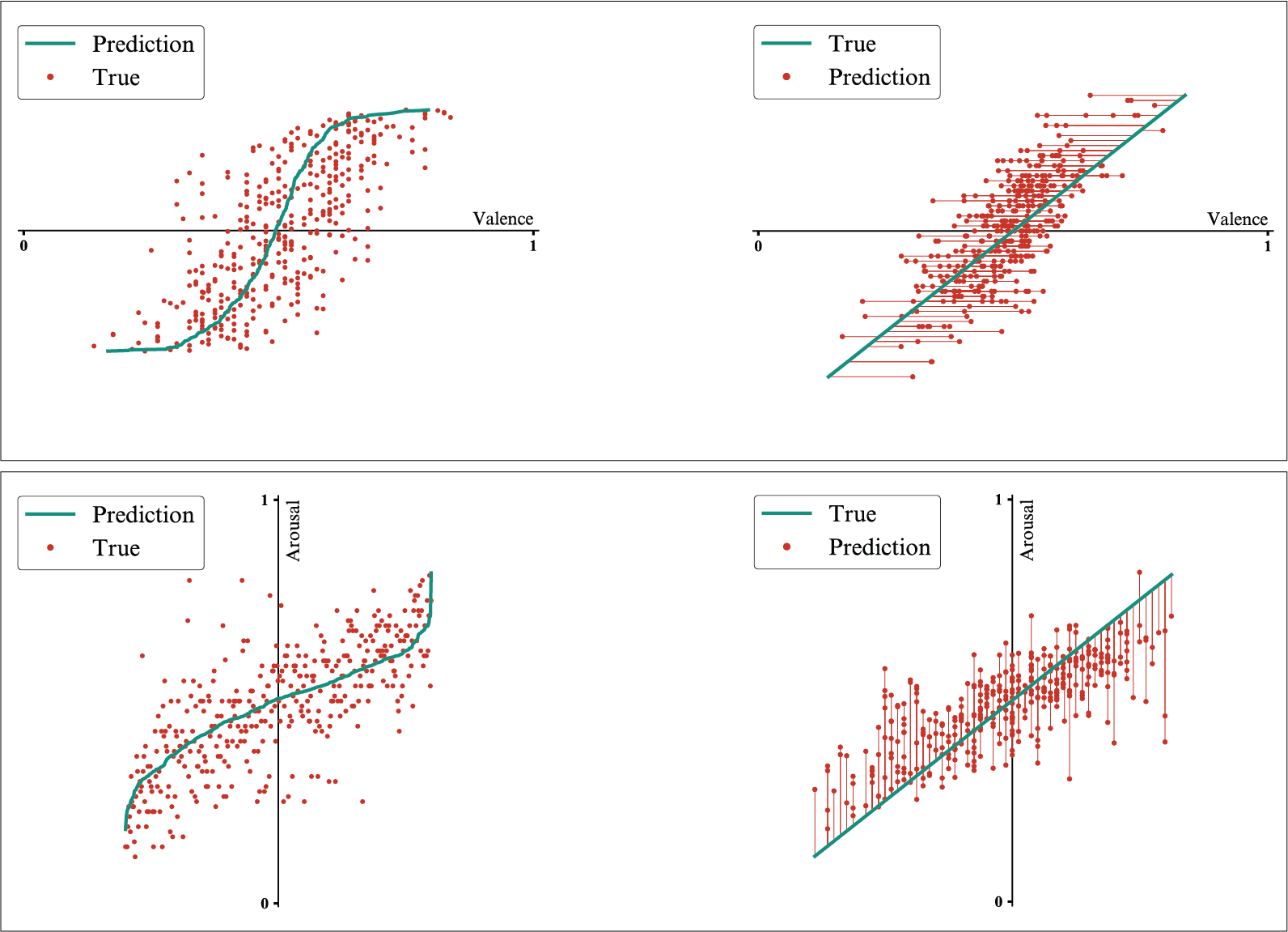
1D-output models trained on the augmented dataset - Results for the valence dimension (top) and for the arousal dimension (bottom).
Pairing these plots with the ranges the predicted values fall in, it is noticeable that the predictions made using the 1D-output CNNs cover a wider range of values that is getting closer to the one defined by the observed values than the predictions made by the 2D-output model.

Augmented dataset - Ranges of the observed and predicted values for 2D-output and 1D-output models.
This spread also shows in the visualization of the predictions in the four quadrants defining the space of emotions, especially in the case of the underrepresented quadrants. While predicting using the 2D-output model leads to accuracy of 22.92% and 32.63% for quadrant 2 and quadrant 4, respectively, the predictions made by the two 1D-output models raises the accuracy to 48.96% and 47.37%, respectively.
Augmented datast - Result for valence and arousal in the space of emotions described by the four quadrants for the 2D-output model (left) and the 1D-output models (right).
In order to understand better of the effect the imbalance in data distribution has when training a neural network, this section presents a comparison between the configurations that led to the best results for each approach to working with the DEAM dataset —original and augmented. As observed above, in both cases —working with the original dataset and augmenting the dataset before training— the configurations composed of two 1D-output models, each predicting in one of the dimensions defining the emotion space, performed better.
For a facile distinction between the two configurations, the models trained on the original dataset are referred by CNNs 1.o. and the models trained on the augmented dataset are announced by CNNs 1.a..
The first analysis method consists in computing the accuracy of predictions made using each configuration in the four quadrants. This represents a numerical translation of the plots displaying the predictions in the emotion space. It can easily be observed that, while the models trained on the augmented dataset led to significant improvement in predictions in the underrepresented quadrants 2 and 4, the accuracy of the predictions in quadrants 1 and 3 is higher in case of the models trained on the original dataset. Nevertheless, the trade-off of a loss in the accuracy of the overrepresented quadrants is preferred, as it leads to overall balanced and qualitative results.

DEAM dataset - Comparison of the accuracy of the quadrant predictions between the configurations of two 1D-output models trained on the original dataset and the augmented dataset.
Evaluating the models' performance by computing the regression metrics MAE, MSE and R2 reveals again the positive influence augmenting the dataset prior to training has on the learning process. Starting with the coefficients of correlation values, they show a stronger relation between the MFCCs features and both dimensions of emotions in the case of working with the augmented dataset. Significant differences are also noted in the errors values, the predictions made by the CNNs1.a. models being closer to the expected values, therefore recording smaller errors.

Comparison of the performance metrics between the configurations of two 1D-output models trained on the original dataset and the augmented dataset.
It was proved that the imbalance in data distribution has a negative impact on the regression performance, as expected. For a comprehensive understanding of the learning process, it it necessary to evaluate the regression using different tools, from different perspectives. The two dimensions of the emotion —valence and arousal— are influenced differently by a set of audio features. This is addressed by dividing the problem in two tasks and building separate models to predict in each dimension.